Support Vector Machines Kernel Trick Spoon-Feed
09 Feb 2015Introduction
Kernel trick is an important concept in machine learning, which is essential to achieve significantly faster computational speed for kernel method based algorithms. (e.g. SVMs, kernel KNN, kernel regression, etc.) In this post, I’d like to introduce in the context of Support Vector Machines 1)why do we need kernel trick, 2)how is it derived step by step, and 3) how does it help to reduce computation complexity.
SVMs Basics
SVMs are computational algorithms that construct a hyperplane, or a set of hyperplanes, in a high or infinite dimensional space. Intuitively, separation between two linearly separable classes is achieved by any hyperplane that provides no misclassification for all data points of any of the considered classes. However, there are many hyperplanes that might classify the same set of data as can be seen in figure 1 (based on a figure from Thomé, 2012)
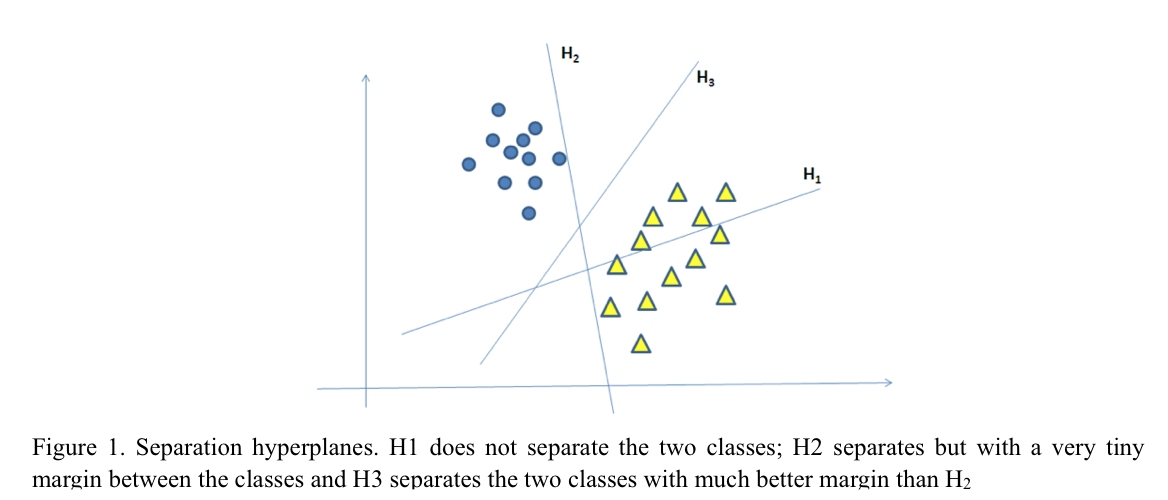
SVMs are an approach in which the objective is to find the best separation hyperplane. That is, the hyperplane that provides the highest margin distance between the nearest points of the two classes. That is the reason why SVM is also called maximum margin classifier. This approach, in general, guarantees that the larger the margin is the lower is the generalization error of the classifier (Thomé, 2012).
To find the hyperplane with the largest margin, we first define the hyperplanes as:
$$f(\boldsymbol {x})=\boldsymbol {w^{T}x}+b$$
, where $\boldsymbol {w}$ and b are, respectively, the vector normal to the hyperplane and the displacement of that vector relative to the origin. We classify data for which $f(\boldsymbol {x}) <-1$ as y = -1 and data for which $f(\boldsymbol {x}) > 1$ as y = 1. The margin between these two hyperplanes: $f(\boldsymbol {x}) = 1$ and $f(\boldsymbol {x}) = -1$, is then defined as:
$$m=\frac {2} {\boldsymbol {|w|}}$$
,where $\boldsymbol {|w|}$ denotes the Euclidean norm of vector $\boldsymbol {w}$. Therefore the decision boundary can be found by solving the following constrained optimization problem:
$$\text{minimize }\frac {1} {2} |\boldsymbol {w}|^{2}\\\text{such that }y_{i}(\boldsymbol {w^{T}x_{i}} + b) \geq 1$$
However, if the data is not absolutely linearly separable, the above approach would fail, since no misclassified observations are allowed. To solve this problem, we introduce a slack variable ($\xi_{i}$) to provide some freedom to the system, allowing some samples to not respect the original equations. This is called the “soft-margin” support vector machine(Vapnik, 1995), and the optimization problem becomes:
$$\text{minimize }\frac {1} {2} |\boldsymbol {w}|^{2} + C\sum_{i=1}^{n} \xi_{i}\\\text{subject to }y_{i}(\boldsymbol {w^{T}x_{i}} + b) \geq 1-\xi_{i}, \xi_{i} \geq 0 $$
,where $\xi_{i}$ is a non-negative slack variable that measures the degree of misclassification of the data $\boldsymbol {x_{i}}$, C is a regularization term, which provides a way to control overfitting, and n is the number of observations.
Motivation of kernel trick
Another way to deal with non-linear separable data is to use a non-linear decision boundary. The key idea is to transform data points $\boldsymbol {x_{i}}$ to a higher dimension ($\varphi(\boldsymbol {x_{i}})$) in which the data become linearly separable. This transformation process is called feature mapping. A polynomial feature mapping example is as follows:
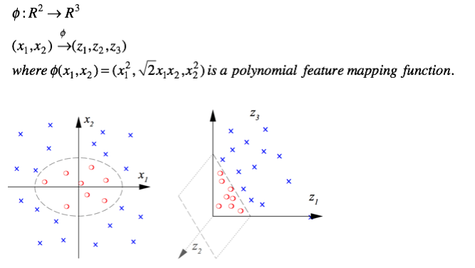
As shown above, mapping the given data from n (with n=2) dimension to m (with m=3) dimensional space helps to achieve linear separability. However, in practice, this mapping process is very computationally expensive when m is large. To avoid computing the coordinates of data in the higher dimensional space explicitly, we employ a kernel trick, which we now explain in detail.
Kernel Trick Derivation Step by Step
First we need some definitions. Defining $\boldsymbol {\varphi}ɸ$ as a non-linear feature mapping function, then the above soft-margin SVM optimization problem becomes:
$$\text{minimize }\frac {1} {2} |\boldsymbol {w}|^{2} + C\sum_{i=1}^{n} \xi_{i}\\\text{subject to }y_{i}(\boldsymbol {w^{T}\varphi(x_{i}}) + b) \geq 1-\xi_{i}, \xi_{i} \geq 0$$
To solve this problem, we can form the Lagrangian:
$L(\boldsymbol {w},b,\xi,a,\lambda) = C \sum_{i=1}^{n} \xi_{i}+ \frac {1} {2} \boldsymbol {|w|}^2 + \sum_{i=1}^{n} a_{i}(1-y_{i}(\boldsymbol {w^{T}\varphi(x_{i})}+b)-\xi_{i}) - \sum_{i=1}^{n} \lambda_{i}\xi_{i}, a_{i} \geq 0, \lambda_{i} \geq 0$
,where $a_{i}$, $\lambda_{i}$, are Lagrange multipliers. Let $\nabla L(\boldsymbol {w},b,\xi,a,\lambda)=0$ we get:
$\boldsymbol {w} = \sum_{i=1}^{n} a_{i}y_{i} \boldsymbol {\varphi(x_{i})} , a_{i} \geq 0$
$\lambda_{i}= C- a_{i} \geq 0 $
$\sum_{i=1}^{n} a_{i}y_{i}=0$
Substituting the above equations back into the Lagrangian, we transform the original optimization problem to:
$L(a,\lambda)= \sum_{i=1}^{n}a_{i} - \frac {1} {2} \sum_{i,j=1}^{n} a_{i}a_{j}y_{i}y_{j}\boldsymbol {\varphi(x_{i})\varphi(x_{j})}$
$\max_{a} L(a,\lambda)$
subject to $0\leq a_{i} \leq C, \sum_{i=1}^{n}a_{i}y_{i} = 0$
This optimization problem is convex, and thus can be solved by many different algorithms such as Coordinate ascent(Vapnik, 1995) and Sequential minimal optimization (SMO)(Shalev-Shwartz, et al., 2013). To identify b, we need to use the Lagrangian again. At the optimal solution, we must have:
$\lambda_{i}\xi_{i} = 0$
$a_{i}(1-y_{i}(\boldsymbol {w^{T}\varphi(x_{i})}+b)-\xi_{i})=0$
If $a_{i} < C$, then $\lambda_{i} = C - a_{i} > 0$ , and thus $\xi_{i}$ must be 0 to make $\lambda_{i}\xi_{i}= 0$. If $a_{i} >0$, then this observation will contribute to the calculation of $\boldsymbol {w}$. Data points with $a_{i} >0$ are thus called support vectors.
$1-y_{i}(\boldsymbol {w^{T}\varphi(x_{i})}+b)-\xi_{i}=0 \Rightarrow b = y_{i}-\boldsymbol {w^{T}\varphi(x_{i})}$
as $y_{i}\in\lbrace -1,1\rbrace$
Taken together, the optimal b can be computed by taking a majority vote of the support vectors as:
$b = \frac {1} {m} \sum_{i=1}^{m} (y_{i}-\boldsymbol {w^{T}\varphi(x_{i})})$
,where m is the number of support vectors.
With the above definitions, we finally are ready to define the "kernel tricks". Suppose we have fit our model's parameters to a training set, and wish to make a prediction at a new input $\boldsymbol {x}$. We would then calculate $\boldsymbol {w^{T}\varphi(x)}+b$, and predict $y = 1$ if this quantity is bigger than 0. But if we substitute $\boldsymbol {w}$ with $\boldsymbol {w} = \sum_{i=1}^{n} a_{i}y_{i}\boldsymbol {\varphi(x_{i})}$, we get:
$$
\begin{equation}
\begin{split}
\boldsymbol {w^{T}\varphi(x)}+b & = (\sum_{i=1}^{n}a_{i}y_{i}\boldsymbol {\varphi(x_{i}))}^{T}\boldsymbol {\varphi(x)} + \frac {1} {m}\sum_{j=1}^{m} (y_{j}-(\sum_{i}^{n}a_{i}y_{i}\boldsymbol {\varphi(x_{i}))^{T}\varphi(x_{j}}))\\
& =\sum_{i=1}^{n} a_{i}y_{i} <\boldsymbol {\varphi(x_{i}),\varphi(x)}> + \frac {1} {m} \sum_{j=1}^{m} (y_{j}-\sum_{i=1}^{n} a_{i}y_{i} <\boldsymbol {\varphi(x_{i}),\varphi(x_{j})}>)
\end{split}
\end{equation}
$$
where $<\boldsymbol {x_{1},x_{2}}>$ denotes the inner product of vector $\boldsymbol {x_{1},x_{2}}$, which is equal to $\sum_{i}^{k}x_{1i}x_{2i}$ with k being the dimension of vector $\boldsymbol {x_{1}}$ and $\boldsymbol {x_{2}}$.
As we can see from the above equation, in order to make a prediction we only need to compute the inner product between the new observation x and support vectors as well as the inner product between the support vectors. This property makes the "kernel trick" applicable to SVMs.
Computation Complexity Reduction by Kernel Trick
We define a function $K(\boldsymbol {x,z})$, such that $K(\boldsymbol {x,z}) = <\boldsymbol {\varphi(x),\varphi(z)}>$. Therefore, the above equation becomes:
$\boldsymbol {w^{T}\varphi(x)} + b = \sum_{i}^{n}a_{i}y_{i}K(\boldsymbol {x_{i},x}) + \frac {1} {m} \sum_{j=1}^{m} (y_{j}-\sum_{i=1}^{n} a_{i}y_{i}K(\boldsymbol{x_{i},x_{j}}))$
In this case, $K(\boldsymbol {x,z})$ is called a kernel function (which must be positive semi-definite), and each kernel function corresponds to a specific feature mapping function. For example, if we define $K(\boldsymbol {x,z}) = (\boldsymbol {xz})^{2}$, then for $\boldsymbol {x}$ and $\boldsymbol {z}$ in $R^{2}$, we have:
$$
\begin{equation}
\begin{split}
K(\boldsymbol{x,z}) & = (x_{1}z_{1} + x_{2}z_{2})^{2}\\
& =x_{1}^{2}z_{1}^{2} +x_{2}^{2}z_{2}^{2} + 2x_{1}z_{1}x_{2}z_{2}\\
& =(x_{1}^{2},\sqrt{2}x_{1}x_{2},x_{2}^{2})^{T}(z_{1}^{2},\sqrt{2}z_{1}z_{2},z_{2}^{2})\\
& =\boldsymbol {\varphi(x)^{T}\varphi(z)}
\end{split}
\end{equation}
$$
where $\boldsymbol {\varphi: R^{2} \rightarrow R^{3}}$
$(x_{1},x_{2}) \rightarrow (x_{1}^{'},x_{2}^{'},x_{3}^{'}) = (x_{1}^{2},\sqrt{2}x_{1}x_{2},x_{2}^{2})$
As shown above, $K(\boldsymbol {x,z}) = (\boldsymbol {xz})^{2}$ corresponds to a feature mapping from $R^{2}$ to $R^{3}$. If we replace $<\boldsymbol {\varphi(x),\varphi(z)}>$ with $K(\boldsymbol {x,z})$, we are able to compute the inner product of features in 3 dimensional space without computing the corresponding coordinates of the 2D features in the 3D space first. This is called the "kernel trick", which helps reduce the computational complexity.
The computation time saved by the kernel trick becomes significant when the features are mapped to a very high dimensional space. Let’s illustrate this by applying a simple RBF kernel function $K(\boldsymbol {x,y})$ to points in $R^{2}$.
$$ \begin{equation} \begin{split} K(\boldsymbol {x,y}) & = exp(\boldsymbol {-(x-y)^{T}(x-y)})\\ & = exp(-x_{1}^{2} + 2x_{1}y_{1}-y_{1}^{2} - x_{2}^{2} + 2x_{2}y_{2}- y_{2}^{2})\\ & =exp(-\boldsymbol {x^{T}x})exp(-\boldsymbol {y^{T}y})exp(2\boldsymbol {x^{T}y})\\ & =exp(-\boldsymbol {x^{T}x})exp(-\boldsymbol {y^{T}y})\sum_{n=1}^{\infty} \frac {2(\boldsymbol {x^{T}y})^{n}} {n!}\\ & =\sum_{n=0}^{\infty} ((\sqrt[n] {\frac {2exp(-\boldsymbol {x^{T}x})} {n!}}\boldsymbol {x})^{T}(\sqrt[n] {\frac {2exp(-\boldsymbol {y^{T}y})} {n!}}\boldsymbol {y}))^{n} \end{split} \end{equation} $$
Therefore, the above RBF kernel corresponds to a mapping from 2 dimensional space to infinite dimensional space. We resort to the kernel trick to do the mapping implicitly since it’s computationally impossible to map explicitly.
References:
- Thomé, Antonio Carlos Gay. SVM Classifiers – Concepts and Applications to Character Recognition. Advances in Character Recognition. November 7, 2012.
- Vapnik, V. (1995). "Support-vector networks". Machine Learning 20 (3): 273. doi:10.1007/BF00994018.
- Shalev-Shwartz, Shai, and Tong Zhang. "Stochastic dual coordinate ascent methods for regularized loss." The Journal of Machine Learning Research 14.1 (2013): 567-599.